ECG Data Generator
Available at
This example is located in the folder named ecg_data, and is contained in the Simulink Model file, named ECG_data_gen.slx, for a design able to generate a continuous ECG signal, coming from a matrix included in the folder as well, named A0001.mat.
Info
They were developped for the Eclipse Z7 board, but may be used on NOA Arch 1 as well.
Data
The data comes from PhysioNet, a platform for biomedical research, on which are published, among other ressources, biomedical data. The data used here contains 12-lead ECG signals, and was taken from a 2020 Cardiology challenge organised by the platform. More precisely, the matrix A0001.mat contains a 15 seconds signal, comes from the China Physiological Signal Challenge of 2018, and can be found on the page referenced above in the folder: training/cpsc_2018.
Another matrix named I0023.mat, that can be used to test the following designs, is also available in the folder. It comes from the St Petersburg INCART 12-lead Arrhythmia Database, can be found on the Physionet page in the folder training/st_petersburg_incart, and lasts 30 minutes.
Structure of the data
Header files named A0001.hea and I0023.hea, are also included: they contain informations on the signals in the .mat files. It is structured in the following way.
For the A0001.hea file for example, from the first line, we see that the recording number is A0001, and the recording file is A0001.mat. The recording has 12 leads, each recorded at 500 Hz sample frequency, and contains 7500 samples.
From the next 12 lines, we see that each signal was written at 16 bits with an offset of 24 bits, 1000 units equal to 1 mV (so 1 unit equals to 1 µV), the resolution of the analog-to-digital converter (ADC) used to digitize the signal is 16 bits, and the baseline value corresponding to 0 physical units is 0. The first value of the signal, the checksum, and the lead name are included for each signal.
From the final 6 lines, we see that the patient is a 74-year-old male with a diagnosis (Dx) of 426783006. The medical prescription (Rx), history (Hx), and symptom or surgery (Sx) are unknown.
All of these informations can be found on the PhysioNet page linked above.
Description
This design has three input ports. The first one activates and deactivates the generation of the signal on the output ports: when its value is zero, the output is nil, and when its value is one, the ECG signal can be read on the output. The second input port controls the sampling frequency of the signal. The third is associated to the factor used to normalize the signal values. The signal is then put on two ports: one interfaced to a DAQ Channel, so that it can be seen on a scope on the generated interface, and the other to a physical analog output of the hardware.
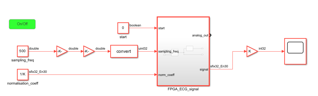
As mentionned before, to manipulate more easily the scaling of the signals at the outputs, the values are normalized before being put on the output ports: they're divided by a factor K, which you can set at 4000 for exemple, as the maximum value in the matrix is 1296. The goal is to have values inside the design between -1 and 1.
On the DAQ channel output, the signal is then multiplied by K, to denormalize it, but you can delete the gain to keep the normalized signal, if needed.
For the analog port, an AnalogOut block is used to scale the input signal to the output voltage. The input signal is in a -1 to 1 range and the output voltage is between -4V and 4V. The amplitude of the original data is divided by 1000, which gives an amplitude resolution of 1 mV instead of 1µV, but allows to view more easily the signals on a small oscilloscope.
This voltage range can of course be modified later through the interface, in the "Analog Outputs" tab of the IOs Setup.
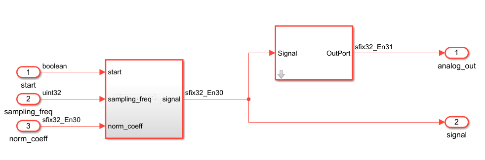
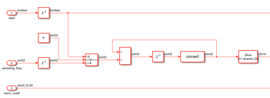
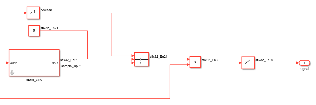
The signal is produced continuously, using a RAM containing the first 1024 values of the first row of the loaded matrix. A counter is used to read these values one by one. The value of the sampling_freq port determines the number of counter cycles needed to go from one value to the next.
Note that the signal chosen here corresponds to the ECG lead I, mesured on the limbs of the patient, more precisly with electrodes placed on both arms.
Note
You may change the signal produced by modifying the content of the memory in the subsystem shown below. You can for example view one of the other 11 signals, or a signal from another array of ECG data.

Ports
| Port | Direction | Interface Type | Description |
|---|---|---|---|
start |
input | AXI4-Lite | on/off signal(boolean) |
sampling_freq |
input | AXI4-Lite | value of the sampling frequency of the output signal; default is 500Hz (uint32) |
analog_out |
output | Analog Output 0 | the output ECG signal, redirected to an analog port (sfix32_En22) |
signal |
output | DAQ Channel 0 | the output ECG signal, redirected to the host computer (sfix32_En21) |
Simulink Interface
First, in the Matlab command window write period = num, where num is the working period corresponding the frequency set later in step 1.4 of the Generation of the Bitstream file process. The blocks in the design work at the period named "period", so it is necessary, to have the design work at the proper frequency.
To implement this design on hardware, you'll also need to load the matrix in your Matlab workspace, by typing the following code in the command window:
load("A0001.mat")
The content of the matrix should appear in your workspace under the name "val".
Do not forget to set the value you want for the constant K, used to normalize the data.
Then you'll need to follow the steps in the Generation of the Bitstream file page, to generate the bitstream file and the interface.
Once this is done, the Simulink interface will look like this:
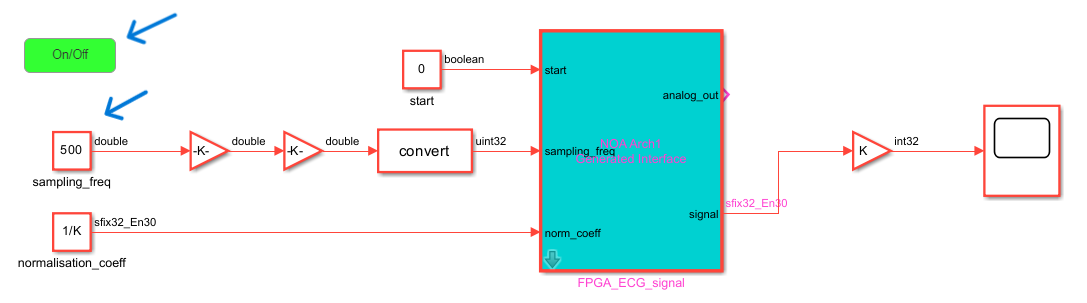
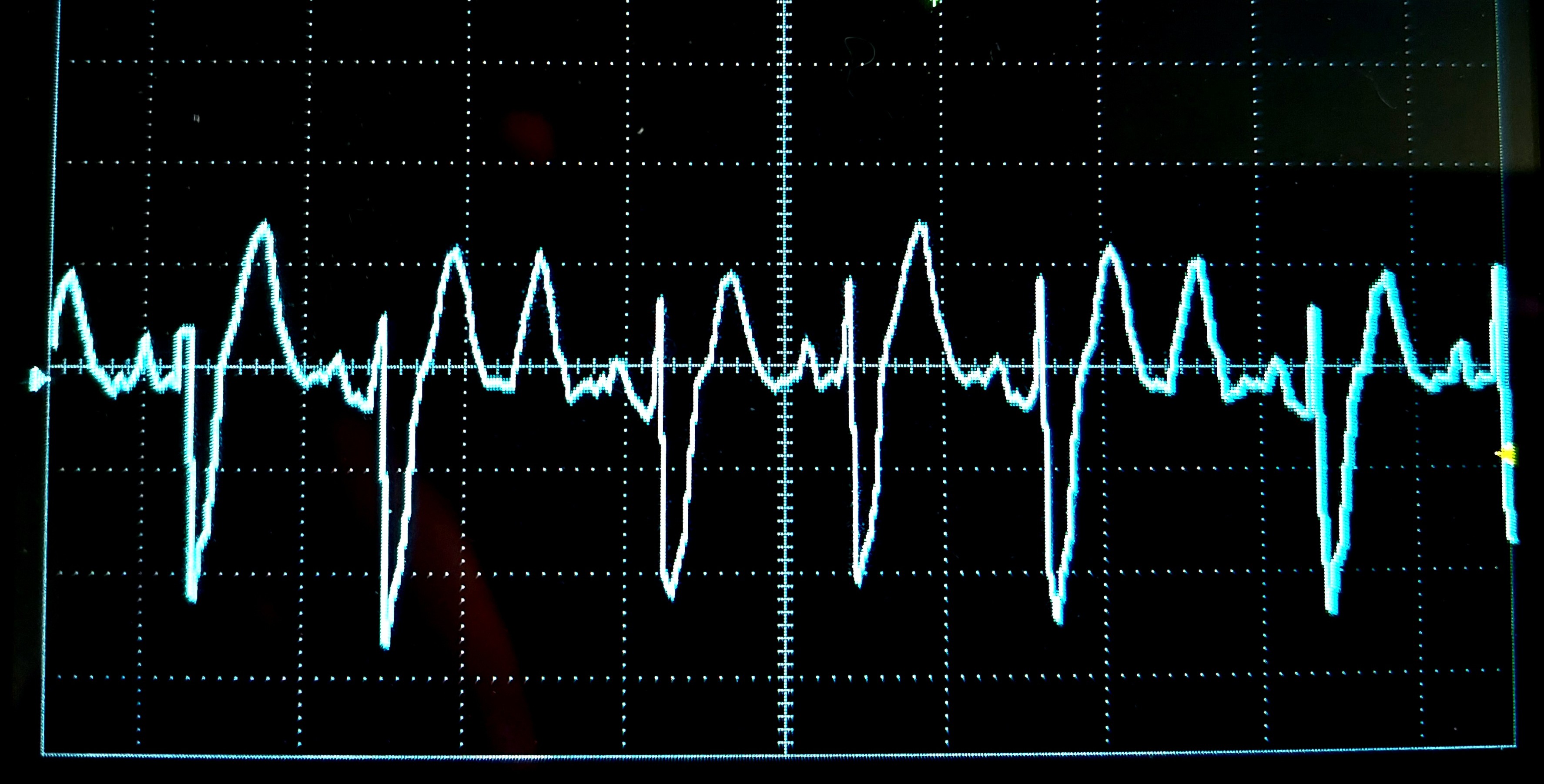
Follow the steps presented on the Connection to the device page, and you will be able to visualize in live on the scope (on the right of the interface), the signal produced on your board (do not forget the settings for the scope). You will also be able to visualize it on an oscilloscope, connected to the first analog port of your device, as shown below.
You can activate or deactivate the output signal by clicking on the green On/Off button, which will change the value of the constant block above on the left to 1 or 0. Modifying the constant block below on the left will change directly the sampling frequency of the output.